Originally posted on Red Hat Developer. This is Part 3 of a three-part series on distributed AI inference. See also Part 1: Core Concepts and Scaling Dimensions and Part 2: Advanced Deployment Patterns. The full article is also available as a single post.
Authors: Fatih Nar, Yuchen Fama, Greg Pereira, Yuan Tang
Reviewers: Taneem Ibrahim, Robert Shaw, Ron Haberman, Anish Asthana
7. Deployment Blueprints by Traffic Shape
The technique sections in Part 1 and Part 2 are the tools; this section shows how they assemble into deployments. Each blueprint follows the same structure (workload signature, KPI priority, topology, the vLLM and llm-d mechanisms it leans on, and a note on cost shape), and should be read as a starting point rather than a prescription.
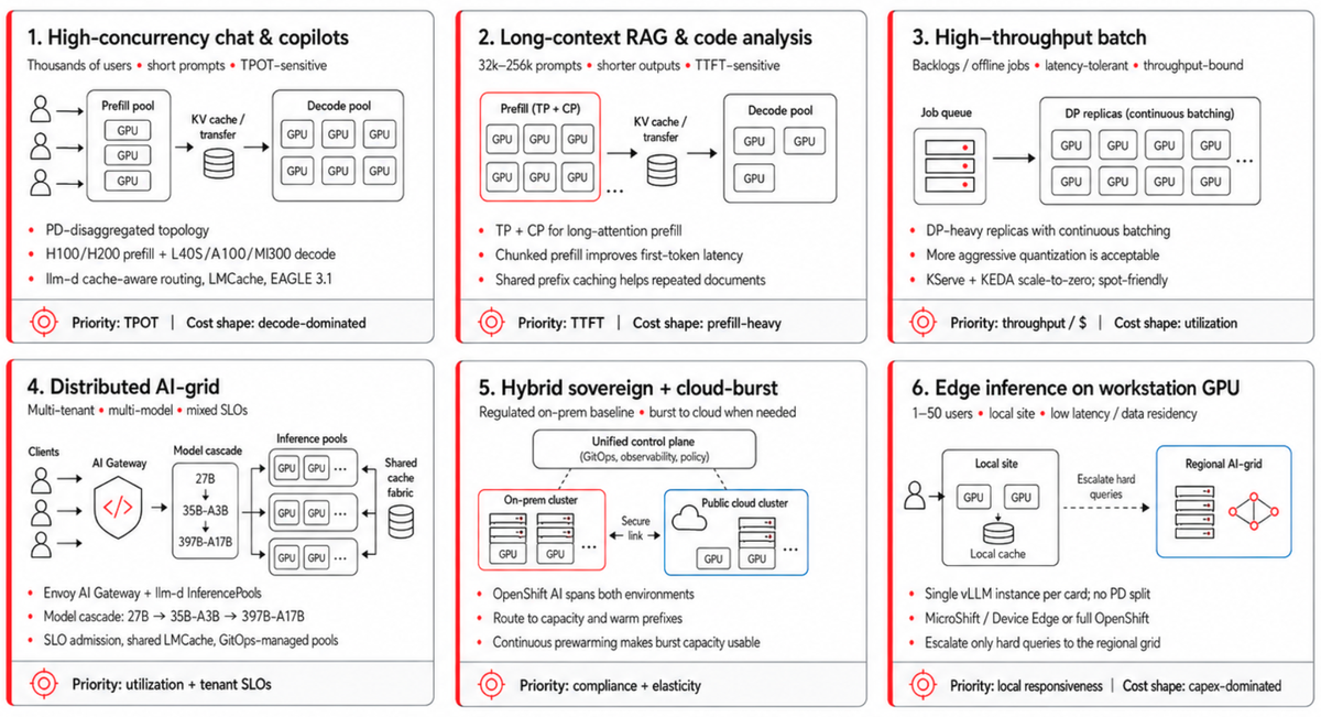
Figure-7 Deployment Blueprints by Traffic
7.1 High-concurrency conversational chat and copilots
Signature. Thousands of concurrent users, prompts in the low hundreds of tokens, outputs of similar length, high prefix reuse from system prompts and few-shot exemplars, and TPOT-dominated SLOs.
Topology. The deployment is PD-disaggregated, with a large prefill pool on cost-optimized GPUs such as H100s and more HBM-capable hardware such as H200/B200-class GPUs as the decode pool especially for long context workloads, where cache-aware routing via the llm-d scheduler pins each session to the decode worker holding its warm KV. EAGLE 3.1 runs on the decode workers, and LMCache offloads from HBM to pinned DRAM (and to NVMe for the longest-tail conversations) so that the decode pool’s effective cache becomes several times larger than its HBM. On the prefill side, chunked prefill (stall-free scheduling) prevents a long prompt from blocking the short ones queued behind it. At the front door, prompt compression on system prompts, debouncing and request coalescing for chatty UIs, and output token caps protect the fleet from runaway generation. The cost shape is decode-dominated, so right-sizing the decode pool is where most of the $/Mtoken savings live.
7.2 Long-context RAG and code analysis
Signature. Lower concurrency than chat, prompts of 32k–256k tokens, outputs in the hundreds, and TTFT-dominated SLOs, because users are waiting for the first useful token of an answer over a long document.
Topology. TP within the node and PCP across GPUs for the prefill phase, so the O(n²) attention work is split rather than left to blow HBM on one device. The decode pool stays small; this workload is bound more by prompt length than by concurrency.
Two things buy back TTFT here, and chunked prefill is not one of them. PCP amortizes the prefill compute across devices; prefix caching skips it outright when the document has been seen before. Chunked prefill, on by default in vLLM V1, earns its keep elsewhere: it keeps one long prefill from starving the decode steps of every other request sharing the GPU. On the long prompt itself it adds a little overhead, and prefix caching becomes the whole game: the warm prefix lives in a shared cache pool any decode worker can reach, so the second pass over a contract never re-prefills it.
The cost shape is prefill-dominated, so the biggest lever on $/Mtoken is prefix-cache hit rate: every avoided re-prefill of a long document is a direct saving.
7.3 High-throughput batch (summarization, labeling, embeddings pipelines)
Signature. Latency-tolerant, throughput- and dollar-bound, typically running overnight on backlogs.
Topology. The pattern is DP-heavy, with as many replicas of the model as fit the budget and each replica running continuous batching maxed out. PD disaggregation tends to buy nothing here, because the wall-clock per request does not matter, so the transfer hop is not worth it. Continuous scheduling, which differs from continuous batching by letting the engine reorder requests to keep batches full even when arrival is bursty, is the right policy. Dynamic quantization can be tuned more aggressively here than in interactive workloads, because a slightly lower output quality is cheaper than a slightly larger GPU footprint. Scale-to-zero between waves via KServe’s KEDA integration keeps the cluster economical, and the workload is spot/preemptible-friendly because retries on batch jobs are cheap.
The cost shape is pure $/token: with latency irrelevant, every lever (max batching, aggressive quantization, scale-to-zero, and spot capacity) goes toward driving dollars per million tokens down.
7.4 Distributed AI-grid: Model-as-a-Service
Signature. The most architecturally rich blueprint we cover. A platform team serves multiple tenants and multiple models (Qwen3.6-27B for one product, Qwen3.5-35B-A3B for another, Qwen3.5-397B-A17B reserved for the hard queries) across heterogeneous SLOs and bursty traffic, and the deployment becomes a grid rather than a collection of single-purpose pools.
Topology. Each model class lives behind its own llm-d InferencePool, with KServe LLMInferenceService resources tracked in GitOps, and AI Gateway implementations such as Envoy AI Gateway sit at the front door handling tenant authentication, rate limiting, and request classification. A shared LMCache fabric across pools lets system-prompt prefixes be reused across instances of the same model, while KEDA autoscaling runs per request-class rather than per pool, so that a “gold” tenant’s bursty traffic can scale its pool aggressively while a “bronze” tenant on the same model sees slower scale-up.
Three mechanisms make this work, and all three were absent or thin in Part-I.
- Model cascading routes easy queries to the smallest model that can handle them and escalates to the next size only when needed. A cascade of Qwen3.6-27B → Qwen3.5-35B-A3B → Qwen3.5-397B-A17B, with escalation triggered by an inexpensive confidence signal or by explicit tenant policy, can cut cluster cost by 40–60% on workloads where the easy fraction dominates. The cascade itself lives in the gateway rather than inside any single InferencePool, so the routing decision can change without redeploying the model.
- SLO-aware admission control is operationally healthier than queuing requests that will miss their SLO, because the queue itself becomes a tail-latency anchor under load. Gold-tier requests get admitted ahead of silver, silver ahead of bronze, and requests likely to exceed token output limits or hit timeouts are rejected at the gateway with a clear error code rather than allowed to chew through GPU-seconds and then time out anyway.
- Adaptive resource scheduling and hotspot prevention is the layer where llm-d’s scheduler does the routing and cluster-level policy does the resource allocation. Adaptive parallelism (TP↔PP↔hybrid switching as traffic patterns shift), dynamic precision (FP8↔FP4 under thermal or load pressure), continuous prewarming of CUDA graphs via traffic-pattern time-series prediction, and MoE expert rebalancing for hot experts are all early-engineering or research today. An AI-grid design that holds up under those changes treats per-tenant SLO classes and telemetry-driven configuration as first-class concerns from the start, so that the static knobs can be swapped for adaptive ones without re-architecting.
The cost shape of this blueprint is the most non-linear of the six. Done well, it can let a platform team serve many tenants at high utilization; done poorly, it becomes a fragmented zoo of single-tenant pools each running at low utilization, and the difference between those two outcomes is almost entirely a matter of cascading, admission control, and shared cache design.
7.5 Hybrid Sovereign -> Cloud-Burst
Signature. Regulated baseline workload that must run on-premises for data residency, sovereignty, or contractual reasons, with peaks that exceed on-prem capacity and need to burst to a public cloud region without breaking the regulatory posture.
Topology. Red Hat OpenShift AI on Red Hat OpenShift provides a single control plane across both environments, with model artifacts in a shared registry and configuration drift managed by GitOps so that the on-prem and burst clusters stay aligned. llm-d’s Inference Gateway fronts both clusters, and congestion-aware, topology-aware scheduling routes individual requests to whichever cluster currently has capacity and the warm prefix. The burst cluster runs cold most of the time. What makes its capacity usable when the spike arrives, rather than tens of seconds later, is fast, deterministic warm-up: pre-pulled pinned images and kernels and a minimal standing footprint, with predictive prewarming via time-series traffic forecasting layered on as that capability matures (Section 7.4). The aim is for the CUDA graphs and KV pools to be warm before traffic shifts, not after.
The cost shape is a capex-anchored on-prem baseline plus variable cloud opex paid only during bursts. The economics hold only if the burst cluster stays genuinely cold between peaks, so the lever is a fast warm-up, not standing capacity.
7.6 Edge inference on a workstation-class GPU
Signature. A single physical site such as a factory floor, retail location, clinic, branch office, vehicle, or regional data closet, where data residency, latency, or connectivity rule out cloud inference for the baseline workload, and backhaul to a regional cluster (when it exists at all) is expensive or intermittent. Concurrent users are typically in the 1–50 range. Both TTFT and TPOT matter to a human operator, but request volume is low enough that throughput is bounded by a single accelerator rather than by anything in the orchestration layer.
Topology. The pattern is a single vLLM instance per accelerator with no llm-d disaggregation, because the prefill-decode transfer hop costs more than it saves below roughly 100 concurrent sessions. KServe handles the serving lifecycle; the OpenShift footprint follows the site: Single Node OpenShift (SNO) for single-node sites, and multi-node OpenShift for regional installations with a handful of cards. GitOps pins the model artifact across the fleet so the same Qwen3.6-27B build runs in every store, clinic, or branch without per-site drift.
The model fits on 96 GB. The hybrid architecture of Qwen3.6-27B is unusually edge-friendly because three of every four attention sublayers are Gated DeltaNet (a linear-attention variant whose state does not grow with context length), so only 16 of the 64 layers maintain a per-token KV cache, with 4 KV heads at head_dim 256. Per-token KV is therefore roughly 64 KB in FP16 or 32 KB in FP8, several times smaller than a pure-transformer model of comparable parameter count, and after 27 GB of FP8 weights and ~4 GB of working memory the remaining ~65 GB of VRAM holds roughly 2 million tokens of cumulative KV at FP8 KV precision. That budget supports any of: ~50 concurrent sessions at 32k context each, ~15 sessions at 128k each, or ~4 sessions at 512k each (the last with FP4 KV). For larger models the envelope tightens quickly: Qwen3.5-35B-A3B at FP8 leaves around 55 GB for KV (workable for moderate concurrency), while Qwen3.5-397B-A17B will not fit a single card at any production precision because the full expert table must be resident.
Hardware is substrate, not strategy. The accelerators at this tier (workstation cards such as the NVIDIA RTX PRO 6000 (96GB) Blackwell, or deskside superchip systems such as DGX Spark and the Supermicro Super AI Station) differ mainly in memory bandwidth and capacity, but the software approach is the same across all of them: quantize to fit one accelerator, serve a single vLLM instance, and scale with replicas (DP) before sharding. The one constraint they share is the absence of NVLink-class fabric between boxes, so any multi-box scale-out is a capacity play built on pipeline or expert sharding, not a tensor-parallel throughput play (see Part 1, Section 3). Decode is memory-bandwidth-bound, so the deployment is capex-dominated, and there is no clean $/MToken story until a site outgrows ~100 concurrent sessions and starts to look like a regional cluster.
Multi-tier pattern. For edge sites that occasionally see queries too hard for the local model, route them over backhaul to a regional cloud cluster running the Section-7.4 AI-grid, with model cascading at the local gateway keeping the fast path on-device and escalating only when a confidence signal or explicit policy demands the flagship model. p99 latency on local queries stays predictable while the heavier model remains available for the long tail, and the backhaul cost stays bounded because escalations are a fraction of total traffic.
8. Inference Troubleshooting Recipes
When TTFT or TPOT regress, the first move is not to change anything but to look at the metrics the fleet already emits, because most regressions point at themselves once you know which dial to read. The vLLM Prometheus endpoint exposes per-request and per-batch metrics (queue time, scheduling delay, prefill duration, decode duration, KV-cache utilization), and the llm-d scheduler emits routing decisions and per-worker queue depths, so the two together answer the first question every time: is the regression at the gateway (routing), in the prefill phase, in the decode phase, or in the KV transfer between them?
For deeper investigation, Nsight Systems captures end-to-end traces and is the right tool when a regression appears to span multiple processes or involves CPU↔GPU coordination, while Nsight Compute drills into a specific kernel when a single operation is the bottleneck.
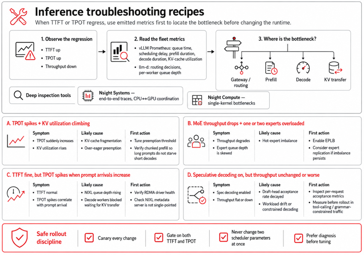
Figure-8 Troubleshooting Recipes
The recipes that recur most often in production inference work are these:
- Sudden TPOT increase with KV utilization climbing usually means KV-cache fragmentation or over-eager preemption; tune the preemption threshold and verify chunked prefill is enabled if long prompts are starving the short decodes queued behind them.
- MoE traffic with degraded throughput and one or two experts at much higher queue depth than the others is hot-expert imbalance; enable EPLB, and if the imbalance persists consider expert replication.
- A disaggregated fleet with TTFT fine but TPOT spikes correlated with prompt arrival means NIXL queue depth is rising and decode workers are blocked waiting for KV transfer; verify RDMA driver health and check that the NIXL metadata server isn’t single-pointed.
- Speculative decoding enabled and throughput unchanged or worse usually means draft-head acceptance rate has decayed; inspect per-request acceptance metrics, because the model or workload may have drifted away from what the draft was trained for.
Roll out changes via canary, gate on both TTFT and TPOT, and never change two scheduler parameters at once, because debugging which one mattered is harder than the original problem.
9. Where to start, where to grow
A practical sequence for a team standing up vLLM and llm-d on OpenShift AI runs roughly like this.
- Begin on a single node with a single vLLM instance, pick the model and the parallelism layout from the Part 1 parallelism table, and baseline TTFT and TPOT on production traffic for at least a week, because the numbers from that baseline are what every later decision will be measured against.
- Add llm-d when the single-node fleet stops scaling linearly: the signal is that a second replica behind a load balancer produces less than 1.8× the throughput of one, which means round-robin routing is leaving cache hits on the table.
- Disaggregate only when the measured prefill-to-decode imbalance is large enough to pay for the transfer hop, because disaggregation done prematurely costs more than it saves; layer speculative decoding once concurrency has stabilized, since at low concurrency the wins are largest and at saturated high concurrency they shrink.
- Reach for the AI-grid blueprint when the platform serves more than one model class to more than one tenant, because the mechanisms (model cascading, SLO classes, shared cache fabric, GitOps-managed pools) earn their complexity at the multi-tenant scale and waste effort below it.
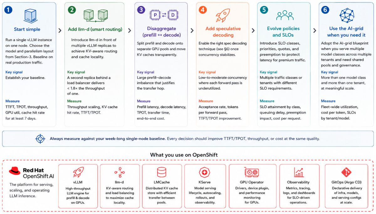
Figure-9 Where to start, where to grow.
The through-line connects every step. Part 1 covered the foundational concepts; Part 2 turned those into optimization levers; this article assembled them into deployments, adding one mechanism at a time and only when a measurement shows the simpler setup has run out, then re-baselining after each change so the next decision rests on data rather than expectation. Start simple, measure honestly, and identify optimization starting from the workload rather than let the technique catalog decide what comes next.
Each rung of that ladder maps to a layer of the Red Hat stack you can deploy rather than assemble by hand. Red Hat OpenShift provides the Kubernetes substrate; Red Hat OpenShift AI adds the model registry, pipelines, monitoring, and governance; Red Hat AI Inference Server packages a hardened vLLM with pinned kernels and LLM Compressor for quantization; KServe manages the serving lifecycle; and llm-d, now a CNCF Sandbox project, supplies the distributed inference layer for cache-aware routing, disaggregation, and KV-cache-aware scheduling. The blueprints in Section 7 are assembled from these building blocks, and the sequence above is how you adopt them without paying for complexity before the workload calls for it.
To learn more, take a look at these resources:
- Designing Distributed AI Inference: Core Concepts and Scaling Dimensions (Part 1 on Red Hat Developer covering prefill/decode phases and 5D parallelism)
- Optimizing Distributed AI Inference: Advanced Deployment Patterns (Part 2 on Red Hat Developer covering P/D disaggregation, KV cache, and speculative decoding)
- Why vLLM is the best choice for AI inference today (Part-I of this series)
- llm-d, the Kubernetes-native distributed inference framework (now a CNCF Sandbox project)
- Combining KServe and llm-d for optimized gen-AI inference
- What GPU kernels mean for your distributed inference (the companion piece on kernels and supply-chain discipline)
- Red Hat AI Inference Server Technical Deep Dive
- LLM Compressor for producing and validating quantized models
- vLLM context-parallel deployment and disaggregated prefilling documentation