Originally posted on Red Hat Developer. This is Part 2 of a three-part series on distributed AI inference. See also Part 1: Core Concepts and Scaling Dimensions and Part 3: Blueprints & Troubleshooting. The full article is also available as a single post.
Authors: Fatih Nar, Yuchen Fama, Greg Pereira, Yuan Tang
Reviewers: Taneem Ibrahim, Robert Shaw, Ron Haberman, Anish Asthana
4. P/D Disaggregation as a Deployment Pattern
Part 1 described disaggregation as a feature of llm-d, but in practice it is a deployment topology (the most consequential one we cover here), and we need to reason about it as such rather than check it off as a capability.
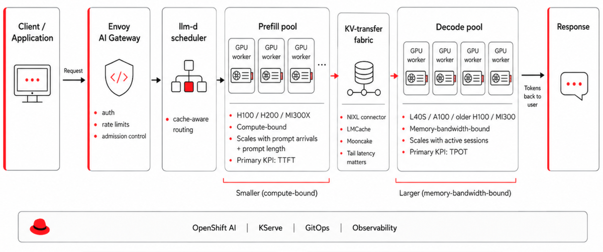
Figure-4 Prefill/Decode
When to disaggregate. The decision rule is neither “always” nor “for big models,” but determined from measurable observations within the system. Profile a baseline single-pool deployment and measure the ratio of prefill GPU-seconds to decode GPU-seconds on your real traffic, then compare it to the ratio of decode-optimized to prefill-optimized GPU cost in your environment. If your traffic is prefill-heavy while you are paying for decode-class hardware (because decode dominates wall-clock), or vice versa, the gap between those two ratios is the upside available from disaggregation. The decision tends to pay off for long-prompt RAG with short answers (prefill-heavy), for high-concurrency chat with short prompts and long answers (decode-heavy), and for any fleet large enough that the $/Mtoken reduction justifies the operational complexity. In our benchmarks that reduction runs 25–40% on chat- and RAG-shaped traffic, consistent with published disaggregation results: Splitwise reports about 20% lower cost at 1.4× throughput, and DistServe up to 7.4× higher goodput. It tends not to pay off for single-node deployments where the network hop between prefill and decode workers would exceed the savings, nor for any fleet small enough that two pools of one are worse than one pool of two.
Sizing the two pools. Prefill workers scale with the arrival rate of new prompts and with prompt-length distribution, while decode workers scale with concurrent active sessions, average token output sizing and target TPOT, and the two scale independently. A useful first cut for a chat workload with mean prompt 800 tokens and mean output 200 tokens at 5,000 concurrent sessions on Qwen3.5-35B-A3B works out to roughly one H100 of prefill capacity per ~30 requests/second of arrival rate, and roughly one decode GPU (L40S-class) per ~150 concurrent sessions, in our lab measurements. These numbers move with model and quantization, but the ratio (typically 1:3 to 1:5 prefill to decode workers for chat) is broadly stable across the workloads we have benchmarked.
KV-transfer connectors and the data path. Once the pools are split, the KV cache produced by prefill must reach decode workers, and vLLM exposes a KVConnector interface with three production-relevant implementations.
| Connector | Best for | Transport | Notes |
|---|---|---|---|
| NixlConnector | Single-cluster, RDMA/NVLink available | NVIDIA NIXL over UCX | Default for high-performance PD; metadata server is a startup SPOF |
| LMCacheConnector | Cross-instance cache sharing, HBM→DRAM→NVMe tiering | NIXL under the hood, plus offload backends | Adds tiered KV cache + shared prefix index (LMCache, arXiv:2510.09665) |
| MooncakeConnector | Cluster-scale shared cache pools | RDMA-native | Best when you want a separate KV-cache cluster that many vLLM instances pull from |
| MooncakeStoreConnector | Tiered cache offloading through use of a distributed master store | Cache offloading | Offload tier behind MooncakeConnector; KV lands in a distributed master store rather than peer HBM |
Table-3 KV-Cache Connectors
Treat the KV-transfer fabric the way you would treat any other production data path: measure end-to-end latency including queue time, alert on tail latency rather than mean, and verify RDMA driver health on every node, because NIXL’s asynchronous send/receive is the right primitive for production only if prefill workers are never made to block on decode-side acknowledgement.
The disaggregated KV cache pool. We find the most useful framing is to stop thinking of the cluster’s KV cache as per-worker memory plus a transfer protocol, and start treating it as a cluster-wide resource with its own scheduling concerns. LMCache makes this explicit by tiering across HBM, DRAM, and NVMe and exposing a global prefix index, so that when two requests share a prefix (a system prompt, a few-shot prefix, the first thousand tokens of a contract), they share KV blocks no matter which instance generated them.
The llm-d scheduler. Cache-aware routing is what turns disaggregation from a feature into a working pattern, because instead of round-robin across decode workers, llm-d routes a request to the worker that already has the warmest KV state for the request’s prefix. Published llm-d benchmarks report up to 57× faster TTFT and 2× throughput against round-robin routing under high prefix reuse (8 pods / 16×H100). Our internal measurements are more conservative, and illustrative rather than guaranteed: a roughly 25% improvement on defaults, 2–3× tokens-per-second-per-GPU when paired with prefix-cache-hit routing, and 3–5× cost-per-token reduction on chat-shaped workloads where prefix reuse is high. Numbers in any given production deployment will be lower than these lab-style figures, though the direction is reliable across every workload we have measured.
Hybrid GPU-CPU prefill. A forward-looking pattern is emerging on Grace Hopper and Vera Rubin superchips, where the CPU side of the superchip handles parts of the prefill (notably embedding lookup and some attention prep) while the GPU handles the matmul-heavy portions. It is not yet a first-line recommendation for production, but it is worth designing the deployment with the prefill pool as a separately scheduled component, so that the worker type can change as the hardware matures without re-architecting.
Failure modes that bite in production. The NIXL metadata server is a single point of failure on startup, so run two behind a TCP load balancer and verify failover before the first canary. Decode workers that fall behind the KV transfer become tail-latency anchors for the whole fleet, which is why admission control at the gateway is more useful than retrying after the fact. And canary rollouts for disaggregated fleets should change one pool at a time, with rollback gates on both TTFT and TPOT, so that a regression in either KPI is caught before it spreads.
5. KV Cache: Tiering, Sharing, Squeezing
PagedAttention solved the fragmentation problem inside a single GPU, but the next set of problems lives across GPUs and across the cluster, and they need different tools.
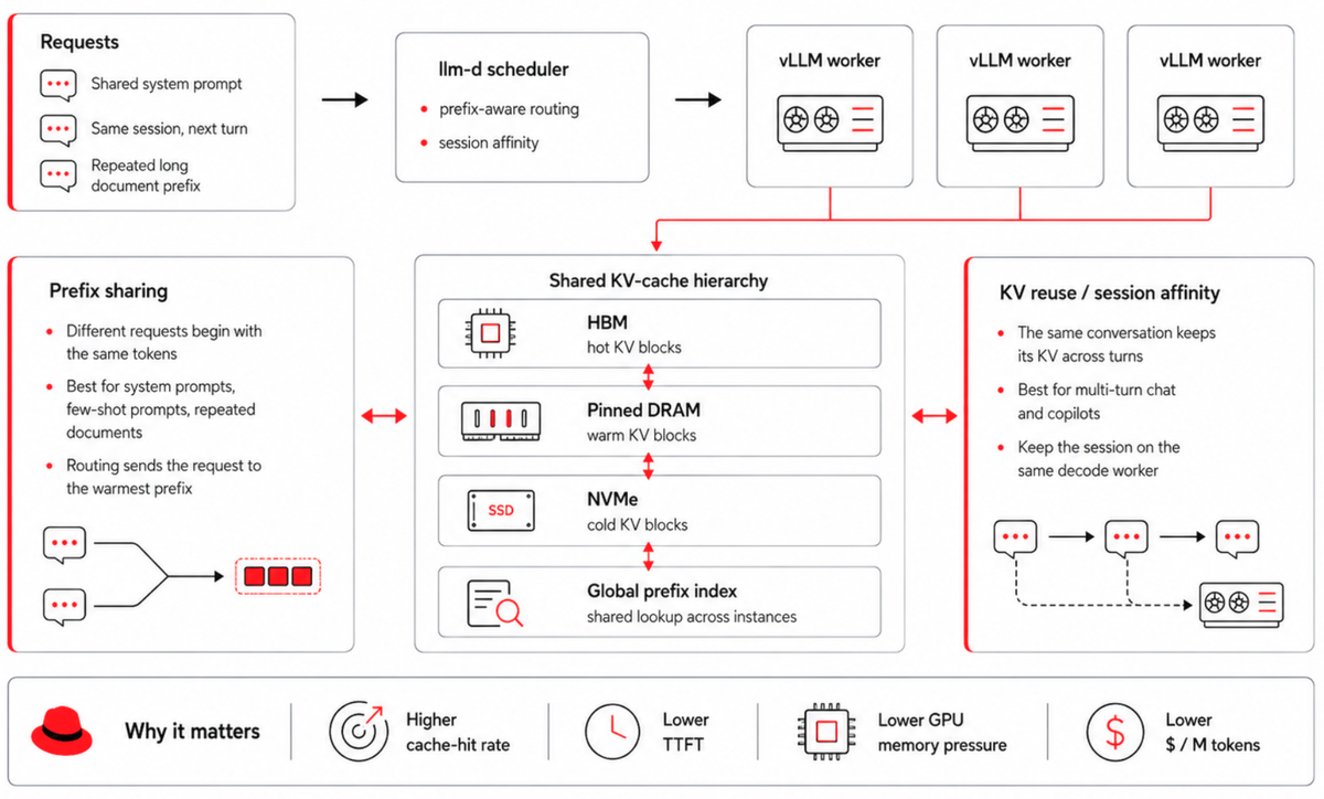
Figure-5 KV-Cache
Tiered hierarchy. Section 4 introduced LMCache’s HBM→DRAM→NVMe tiering as a cluster-wide resource; the question here is when to turn it on. Most enterprise workloads have a long tail of cold prefixes that fit in DRAM or NVMe but not in HBM, and the decision rule is simple: if your prefix-cache hit rate would be substantially higher with a 10× larger cache than you can afford in HBM, then tiering pays for itself.
KV reuse vs prefix sharing. These two are often conflated, but they are different concerns with different configuration knobs. Prefix sharing means that two requests starting with the same tokens share the cache, while KV reuse means that the same request’s KV is retained across turns of a multi-turn session. Multi-tenant chat platforms benefit from both, because shared system prompts give one and conversation history gives the other. Prefix sharing is therefore a routing concern (send the new request to the worker that has the warm prefix), while reuse is a session-affinity concern that keeps the same session pinned to the same decode worker.
Quantization. FP8 KV cache halves the memory footprint with a measurable but usually acceptable quality cost on most enterprise tasks, while FP4 KV is more aggressive and currently best deployed only on workloads where you can afford an evaluation pass against your own data. Red Hat’s LLM Compressor produces quantized variants of the Qwen models and validates them against your own eval set rather than a generic benchmark.
Decode kernels. vLLM’s decode path is fast in 2026 not because of one optimization but because of a family of them, with FlashMLA (DeepSeek), ThunderMLA (Stanford), and PyTorch’s FlexAttention decode path all contributing. Platform teams rarely tune these kernels directly, but knowing which one your vLLM build is using helps when investigating an unexpected decode regression after a version upgrade. At fleet scale the harder problem is provenance and consistency: every prefill, decode, and draft-model replica must load identical, pinned kernel binaries, which is why a production runtime ships them build-from-source and SBOM-covered in the image rather than pulling them from a public registry at first request. We cover that kernel supply-chain trade-off, and the GPU Kernel Manager (GKM) bridge for heterogeneous fleets, in What GPU kernels mean for your distributed inference.
PagedAttention vs Radix-Attention. SGLang’s RadixAttention takes a different architectural bet by organizing the cache as a prefix tree and letting the structure of conversation guide eviction, whereas PagedAttention treats the cache like virtual memory pages, and reasonable engineers disagree on the trade-off: Radix tends to win on workloads with deep, branching prefix trees (agent workflows, structured prompting), while PagedAttention tends to win on workloads with high variance in sequence length and irregular prefix patterns. vLLM has stayed with PagedAttention because the engine is general-purpose and the page-table abstraction generalizes more cleanly to disaggregation, where the unit of transfer is naturally a page.
6. Speculative Decoding
Speculative decoding generates several candidate tokens at once with a cheaper draft path, then verifies them with the target model, so that when the drafts are accepted the model emits several tokens per forward pass. The families of technique that vLLM supports today are worth distinguishing, because their cost profiles are very different.
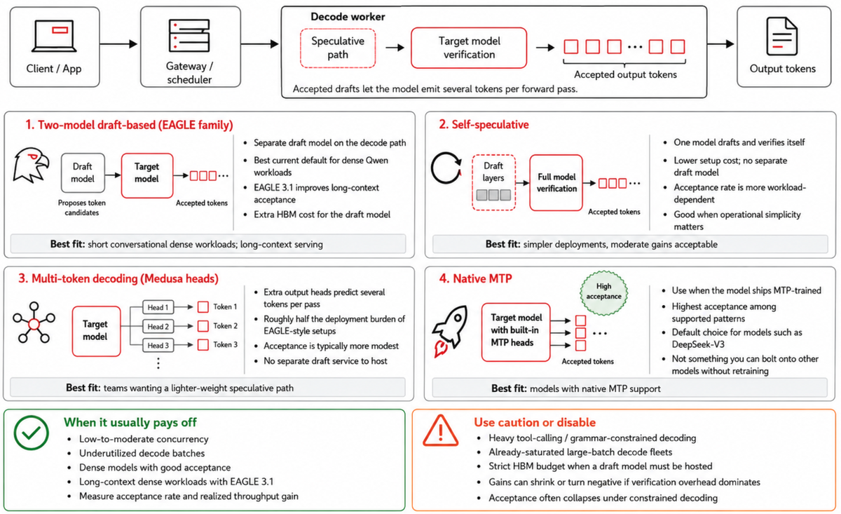
Figure-6 Speculative Decoding
Two-model, draft-based (EAGLE family). A small draft model proposes tokens that the target then verifies. EAGLE-3 has been reported to reach up to ~6× speedups on dense models, while EAGLE 3.1 (May 2026) extends that gain materially into long-context regimes with up to 2× longer acceptance length than EAGLE-3, making it a strong starting choice for dense Qwen3.6 workloads.
Single-model self-speculative. The model drafts and verifies itself, typically by using a subset of its own layers as the draft, which gives a lower setup cost (there is no separate draft model to train or host) at the price of a more variable acceptance rate that depends on the workload.
Multi-token decoding (Medusa heads). Adding multiple output heads to the target model lets it predict several tokens per pass, and although the engineering cost is roughly half that of EAGLE-3 to deploy, the acceptance rates are correspondingly more modest, at around 0.55–0.70.
Interleaved decode and constrained-decoding interactions. Less a technique than a scheduling choice, modern vLLM interleaves spec-decoded sessions with normal decode steps to keep batches full. There is one important caveat: when the workload uses constrained decoding (JSON mode, tool calls with grammars), the acceptance rate of speculative decoding often collapses because the constraint mask invalidates speculative tokens, so measure before assuming spec decoding helps in tool-calling traffic.
Multi-token prediction (MTP). Some models, notably DeepSeek-V3, ship with MTP heads trained jointly with the main model, and acceptance rates exceed 80% out of the box. This makes MTP the natural choice for any model that ships MTP-trained, but it cannot be bolted on to models that don’t without re-training.
| Workload | Anchor model | Recommended | Why |
|---|---|---|---|
| Short conversational, dense | Qwen3.6-27B | EAGLE 3.1 | Best accept-rate/cost ratio, current generation |
| Long-context (>64k) | Qwen3.5 dense or MoE | EAGLE 3.1 | Long-context acceptance is the headline improvement |
| MoE flagship | Qwen3.5-397B-A17B | Native MTP if trained; else EAGLE-3 | Active-param shape favors MTP-style heads |
| Code completion | Qwen3.6 dense | n-gram / prompt-lookup | Repetitive code structure makes hit rate high; no draft to host |
| Strict memory budget | any | n-gram | No draft model to host on decode GPU |
| Heavy tool-calling traffic | any | Disable or test | Constrained decoding interaction is severe |
Table-4 Speculative Decoding Options vs Workloads
Note: The draft model occupies decode-worker HBM and adds verification overhead, so on already-saturated, large-batch decode fleets the win from spec decoding shrinks, because the batch is already amortizing the kernel launch. At the extreme it can become a net loss, so the clearest wins are at low-to-moderate concurrency, where each forward pass is underutilized.
Continue to Part 3: Blueprints & Troubleshooting, which covers six deployment blueprints, troubleshooting recipes, and a scaling roadmap.