Introduction to Scikit Flow

(This blog is featured in DataScienceWeekly here)

In November, 2015, Google open-sourced its numerical computation library called TensorFlow using data flow graphs. Its flexible implementation and architecture enables you to focus on building the computation graph and deploy the model with little efforts on heterogeous platforms such as mobile devices, hundreds of machines, or thousands of computational devices.

TensorFlow is generally very straightforward to use in a sense that most of the researchers in the research area without experience of using this library could understand what’s happening behind the code blocks. TensorFlow provides a good backbone for building different shapes of machine learning applications.

However, there’s a large number of potential users, including some researchers, data scientists, and students who may be familiar with many data science concepts/algorithms already but who never get involved in deep learning research/applications, may found it really hard to start hacking. That’s where Scikit Flow comes in to help.

Scikit Flow is a simplified interface for TensorFlow, to get people started on predictive analytics and data mining. It helps smooth the transition from the Scikit-learn world of one-liner machine learning into the more open world of building different shapes of ML models. You can start by using fit/predict and slide into TensorFlow APIs as you are getting comfortable. It’s Scikit-learn compatible so you can also benefit from Scikit-learn features like GridSearch and Pipeline.

Deep Learning Models

Scikit Flow provides a set of high level model classes that you can use to easily integrate with your existing Scikit-learn pipeline code.

Deep Neural Network

Here’s an example of 3 layer deep neural network with 10, 20 and 10 hidden units in each layer respectively:

import tensorflow.contrib.learn as skflow
from sklearn import datasets, metrics

iris = datasets.load_iris()
classifier = skflow.TensorFlowDNNClassifier(hidden_units=[10, 20, 10], n_classes=3)
classifier.fit(iris.data, iris.target)
score = metrics.accuracy_score(iris.target, classifier.predict(iris.data))
print("Accuracy: %f" % score)

Custom Model

Scikit Flow grows as TensorFlow grows. You can basically insert any TensorFlow code into a custom model function that accepts predictors X and target y and returns predictions and losses, and then pass it to skflow.TensorFlowEstimator. Here’s an example of how to pass a custom model to TensorFlowEstimator, utilizing some built-in losses_ops from Scikit Flow. More advanced examples can be found in examples folder, such as deep residual network that seemlessly uses TensorFlow code.

from sklearn import datasets, metrics

iris = datasets.load_iris()

def my_model(X, y):
    """This is DNN with 10, 20, 10 hidden layers, and dropout of 0.5 probability."""
    layers = skflow.ops.dnn(X, [10, 20, 10], keep_prob=0.5)
    return skflow.models.logistic_regression(layers, y)

classifier = skflow.TensorFlowEstimator(model_fn=my_model, n_classes=3)
classifier.fit(iris.data, iris.target)
score = metrics.accuracy_score(iris.target, classifier.predict(iris.data))
print("Accuracy: %f" % score)

Recurrent Neural Network

Recurrent neural networks is widely used for many areas, such as text classification, sentiment analysis, etc. Using Scikit Flow, all you need to do is to provide some processing function input_op_fn that manipultes the input data into the right shape (we will not cover them here, see examples folder on Github), change a few parameters, and call fit as usual. Currently Scikit Flow provides high level APIs for variants of RNNs.

Various recurrent units, e.g. GRU, RNN, LSTM
Bidirectional RNN
Multi-layer RNN

Example:

classifier = skflow.TensorFlowRNNClassifier(rnn_size=EMBEDDING_SIZE, 
    n_classes=15, cell_type='gru', input_op_fn=input_op_fn,
    num_layers=1, bidirectional=False, sequence_length=None,
    steps=1000, optimizer='Adam', learning_rate=0.01, continue_training=True)

Convolutional Neural Network

Convolutional Neural Network is widely used in areas like computer vision. Here let’s take a look at the MNIST image classification example from TensorFlow tutorial - Deep MNIST for Experts but using more concise interface provided by Scikit Flow. Import statements and additional comments are ignored in this blogpost but you can found them in examples folder. A custom model called conv_model with convolutional and densely connected layers specified is passed into skflow.TensorFlowEstimator. You get all other built-in parameters such as learning_rate and batch_size for free at the same time without getting into writing repeated code using TensorFlow low level APIs.

# Loading MNIST data
mnist = input_data.read_data_sets('MNIST_data')

def max_pool_2x2(tensor_in):
    return tf.nn.max_pool(tensor_in, ksize=[1, 2, 2, 1], strides=[1, 2, 2, 1],
        padding='SAME')

def conv_model(X, y):
    # reshape X to 4d tensor with 2nd and 3rd dimensions being image width and height
    # final dimension being the number of color channels
    X = tf.reshape(X, [-1, 28, 28, 1])
    # first conv layer will compute 32 features for each 5x5 patch
    with tf.variable_scope('conv_layer1'):
        h_conv1 = skflow.ops.conv2d(X, n_filters=32, filter_shape=[5, 5], 
                                    bias=True, activation=tf.nn.relu)
        h_pool1 = max_pool_2x2(h_conv1)
    # second conv layer will compute 64 features for each 5x5 patch
    with tf.variable_scope('conv_layer2'):
        h_conv2 = skflow.ops.conv2d(h_pool1, n_filters=64, filter_shape=[5, 5], 
                                    bias=True, activation=tf.nn.relu)
        h_pool2 = max_pool_2x2(h_conv2)
        # reshape tensor into a batch of vectors
        h_pool2_flat = tf.reshape(h_pool2, [-1, 7 * 7 * 64])
    # densely connected layer with 1024 neurons
    h_fc1 = skflow.ops.dnn(h_pool2_flat, [1024], activation=tf.nn.relu, keep_prob=0.5)
    return skflow.models.logistic_regression(h_fc1, y)

# Training and predicting
classifier = skflow.TensorFlowEstimator(
    model_fn=conv_model, n_classes=10, batch_size=100, steps=20000,
    learning_rate=0.001)

Modelling Techniques

Many data science modelling techniques, including early stopping that’s used very often in Kaggle competition and custom learning rate decay can be used easily.

Early Stopping

You can provide early_stopping_rounds in skflow.monitors.ValidationMonitor object and pass into fit function to monitor the training and stop the training when validation loss stops decreasing for several continuous rounds.

val_monitor = skflow.monitors.ValidationMonitor(X_val, y_val,
                                                early_stopping_rounds=200,
                                                n_classes=3,
                                                print_steps=50)
# classifier with early stopping on validation data
classifier = skflow.TensorFlowDNNClassifier(hidden_units=[10, 20, 10],
                                             n_classes=3, steps=2000)
# provide a validation monitor with early stopping rounds and validation set
classifier.fit(X_train, y_train, val_monitor) 

Custom Decay Function for Learning Rate

Here we give an example of using TensorFlow’s exponential decay function.

# setup exponential decay function
def exp_decay(global_step):
    return tf.train.exponential_decay(
        learning_rate=0.1, global_step=global_step,
        decay_steps=100, decay_rate=0.001)

# use customized decay function in learning_rate
classifier = skflow.TensorFlowDNNClassifier(hidden_units=[10, 20, 10],
                                            n_classes=3, steps=800,
                                            learning_rate=exp_decay)

More features related to modelling techniques are also available such as multi-output regression/classification, custom class weights, dropout probability, batch normalization, etc. We will continue adding more examples on Github in the future.

Additional Features

Scikit Flow provides many additional features to help you easy and streamline your model building experience. It’s evolving very rapidly. We are actively seeking suggestions/ideas and welcoming any pull requests. Join our Gitter to discuss your ideas or drop your feature requests at Github issues.

Flexible Automatic Input Handling

We try to make your life easier with automatic handling of various data types, such as numpy array/matrices, pandas/dask data frames, and iterators.

For example, sometimes when your dataset is too large to hold in the memory you may want to load it into a out-of-core dataframe with the help of dask library to firstly draw sample batches and then load into memory for training.

# We can load data into pandas.DataFrame
X_train, y_train, X_test, y_test = [pd.DataFrame(data) for data in [X_train, y_train, X_test, y_test]]
# Or load data into dask.DataFrame, details see: http://dask.pydata.org/en/latest/dataframe.html
X_train, y_train, X_test, y_test = [dd.from_pandas(data, npartitions=2) for data in [X_train, y_train, X_test, y_test]]

classifier = skflow.TensorFlowLinearClassifier(n_classes=3)

classifier.fit(X_train, y_train)
# Make predictions on each partitions of testing data
predictions = X_test.map_partitions(classifier.predict).compute()
# Calculate accuracy
score = metrics.accuracy_score(y_test.compute(), predictions)

Model Persistence

We try to make it easy for you to save the model every once a while and continue training it any time in the future.

Each estimator has a save method which takes folder path where all model information will be saved. For restoring you can just call skflow.TensorFlowEstimator.restore(path) and it will return object of your class.

classifier = skflow.TensorFlowLinearRegression()
classifier.fit(...)
classifier.save('/tmp/tf_examples/my_model_1/')

new_classifier = TensorFlowEstimator.restore('/tmp/tf_examples/my_model_2')
new_classifier.predict(...)

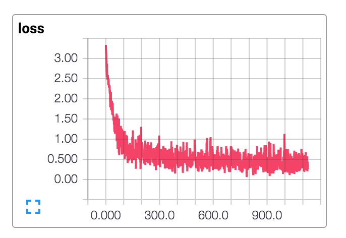
Summaries/TensorBoard

To get nice visualizations and summaries you can use logdir parameter on fit. It will start writing summaries for loss and histograms for variables in your model. You can also add custom summaries in your custom model function by calling tf.summary and passing Tensors to report.

classifier = skflow.TensorFlowLinearRegression()
classifier.fit(X, y, logdir='/tmp/tf_examples/my_model_1/')

Then run next command in command line:

tensorboard --logdir=/tmp/tf_examples/my_model_1

and follow reported url in your console to open the tensorboard.

More Examples and applications can be found on Github:

Text classification (RNN & Convolution, word and character-level)
Digits & MNIST (Conv, more Conv and ResNet)
Language models
Neural Translation Model

More blogposts about Scikit Flow:

More exciting things are happening! Spoiler alert: we are moving to TensorFlow soon! Stay tuned!

Update: skflow has been merged to TensorFlow as its TensorFlow Learn module. Please find most updated examples here.

Banner Credit to TensorFlow Org